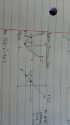
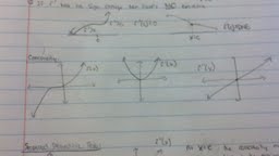
This week in class we learned to compare the graphs of the first derivatives and second derivatives. The tools we use to find anti derivatives in the previous functions are used heavily in this new section. By comparing these graphs we were able to understand the shape of the original function. The methods we learned come in handy when we are not given full information on the original equation. However, this week I struggled with the material. I had a hard time understanding how to solve the problems without the use of the calculator. Much of this confusion had me while I was working on the assignments. I fairly understood the notes in class, however when I started the assignment it was more difficult and the format was different. I understood well how to find requirements in graphs when using the calculator where it would should concavity. I need to get better at using skills without the use of a calculator. Next week, I am guessing I will learn more strategies and comparison between derivatives in graphs that will be good practice without the use of a calculator. I was also confused on all the separate rules in 4.3. I understood the concepts but had a hard time remembering how to solve a problem with using support for the rules. But with help from these two websites I was able to understand the concept a bit better. http://www.math.hmc.edu/calculus/tutorials/secondderiv/ and http://mathworld.wolfram.com/FirstDerivativeTest.html. What I found with the second derivative test is when x=c in a particular graph the concavity would be concave down in the original function due to the graph of the second derivative of c being negative where c is the critical point. The second derivatives can be handy in order to solve the zeros to find the inflection points and whether it is concave up or down. Overall, although I struggled this week I would say I tried my best in participating in what I could do group discussions and homework. This section defiantly was a challenge!
This week, we jumped into the beginning of chapter 4. Chapter 4 consists of using the same processes of derivatives we have used in the past, just additional information. In 4.1 and 4.2 it discussed the properties of extreme values and the mean value theorem. Much of my graphing skills came in handy for this section to interpret the solutions. When solving solutions I learned that much of it was just common sense, like the mean value theorem which states that a point (a,b) is continuous for f(x)=y and differential at every point (a,b). If this statement is true the mean value then states that at least one point c in (a,b) must be the rate of change formula, f(c)= f(b)-f(a) / b-a . At first, I had a hard time understanding what the complex definition meant. However, once I put it to work I began to grasp it better. To show that a function satisfies the mean value theorem the steps to solve it goes like this: You first must find the derivative of the original function. You then need to find the average rate of change by plugging it into the equation with the b and a values. To check you take the derivative equal to the rate of change value to find x. The x of that solution becomes the c value. To find the y coordinate for the c value, plug c back in to the regular function for x to get y. Section 4.2 I understood fairly well. It was the same process of taking anti-derivatives but instead of just leaving the answer as c, we solved for that value. I found this to be easy because it was the same method as what we had our test over in chapter 3 except to find c you plug in the x and y values. My participation I felt was good this week. I have gotten a lot out of the CCC of the homework, and when I am confused on a question or concept I try to go over it or ask for help. Next week, I am as summing we will continue looking at chapter 4 and going further in depth. I ran across some questions on the activity that became a little confusing.
These websites/video are helpful for more information on the MVT: http://www.youtube.com/watch?v=xYOrYLq3fE0 http://tutorial.math.lamar.edu/Classes/CalcI/MeanValueTheorem.aspx This week we finished up the sections in chapter 3. We learned how to imply inverses in dervative trig functions and how to take derivatives involving exponentials and logarthims. These new sections involve using the same dervative methods like before except it involves new equation proofs in order to solve. However the chain rules, product rules, and quotient rules, still apply of taking the dervative of (d/dx). These are important concepts to learn in order to continue learning rules to tak dervatives of more complex functions. This week was a bit easier than last week in dealing with dervatives. Taking the inverses were easier to grasp because I have already had lots of practice in taking dervatives of regular functions. Because of this, it was simple just to use the same methods but including the inverse equation and rules. Taking derviatives of exponentials and logarthiums were also easier to understand because you just had to memorize the certian definitions involved in certain situations in order to solve. The most difficult part of this week was answering more complex problems that delt with all the dervative rules used together. It becomes difficult to sort out which rules and defintions must be used to solve certain problems. Therefore really looking at the equation to the problem and understanding specifically what it is displaying will help sort out what techniques must be used in order to solve the dervative or inverse. For example, when I got my quiz back I was a little disspointed in my score. This was because I thought I understood the concept of dervatives and the rules that delt with them. However, I failed to notice that in some of the problems I had not used the product rule along with the chain rule. With solving for inverses of trig functions you must remember to also use the co inverses also. These co functions are easier to sort out once you memorize or remember the orginal ones of sin, tan, sec. To find csc, cot, and cos you simply take the negative of its oppisite. So in other means the inverse of sin= - cos inverse. Inverse of tan= - cot inverse. Inverse of sec = - csc inverse. Knowing these rules will allow you to take the dervative of inverse trig fucntions by applying the x value given and plugging it into the x value in the equation and following the chain, product, ect rules with dervatives with it to simplify. My participation again this week I thought went well. I particapted in group questions and continued to work on problems I did not understand to where I didabnd asked for help when necessary on assignments. Next week I believe we will continue applying all these techniques and mothods with dervatives with us to carry over into story problems and real life situations. Therefore it will be important for me to continue to do well in understanding all of these dervative rules.
http://tutorial.math.lamar.edu/Classes/CalcI/DiffInvTrigFcns.aspx http://www.sosmath.com/calculus/diff/der08/der08.html |